Implementation
Hardware Setup
We used the Unitree Go2 quadruped robot for this project.
This robot dog comes with four legs, each with 3 motors, resulting in a system with 12 degrees of freedom. It also has a front camera and LiDAR sensor. For this project, we solely relied on the LiDAR sensor to do our mapping, and we used the built-in software for controlling the legs given a translational and rotational velocity. This is possible because the robot legs are capable of maneuvers such as “crab walking” left and right and also pure rotation (with some margin of error) due to their 3-motor design.
Software Design
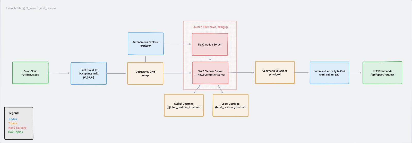
Our system is built on ROS2 and uses the Nav2 library. It starts from one launch file, go2_search_and_rescue. With this launch file, we launch multiple nodes:
- pc_to_og: Point cloud to occupancy grid conversion
- explorer: Autonomous explorer node that checks occupancy grid and publishes new goals based on frontiers
- cmd_vel_to_go2: Controller node that converts between cmd_vel commands to the commands expected by the Go2 software
- nav2_bringup: A launch file that launches all nav2 servers related to planning
The structure of our coordinate frames is as follows:
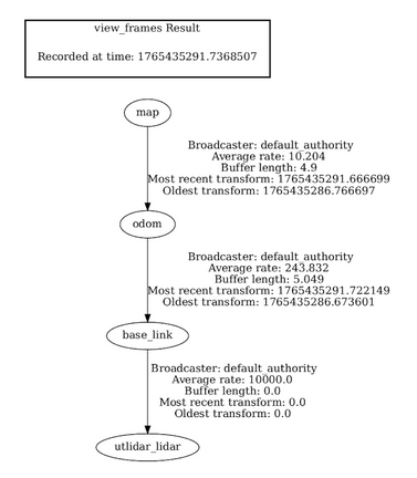
The map frame has a static transform to the odom frame in our case, which we publish as a part of our launch file using ros2’s builtin static transform publisher. The odom frame corresponds to the fixed frame tracked by the odometry of the robot. The base_link frame corresponds to the robot itself, and the transformation between base_link and utlidar_lidar is again another static transform published by our launch file based on the geometry of the robot.
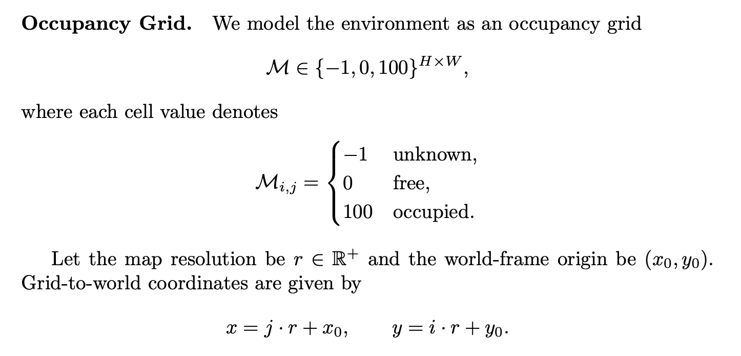
Point Cloud to Occupancy Grid
The Go2 robot publishes point cloud data from its lidar to the /utlidar/cloud topic. From here, our pc_to_og node subscribes to this real-time data and converts it into an occupancy grid. To update this occupancy grid, we use Bayesian log-odds updates by representing each cell in the grid as the log-odds of being occupied. For each point in the point cloud, we:
- Account for the transformation of the LiDAR to the robot because of its slight rotation on the y-axis of the robot when converting between the utlidar_lidar frame and base_link.
- Transform from the robot coordinate system (base_link) to the odom frame, which provides us a fixed point of reference to anchor our map.
- Project these points that are now in the odom frame onto the 2D XY plane.
- Discretize the continuous coordinates on this XY plane into cells following our grid resolution of 0.05m, and height/width of 300 cells.
- In the odom frame, trace a ray from the robot’s current coordinates projected onto the XY plane to the cell corresponding to the current point in the point cloud we’re processing.
- Along the path of the ray, update each cell with a log-odds update with a “free” probability of 0.1. We set this relatively low to help decay dynamic obstacles and noise.
- At the end of the ray, update the cell with a log-odds update with an “occupied” probability of 0.7. We set this relatively high to help rapidly detect new static obstacles.
- At the end of the updates, we clip each cell to be between [-2.0, 3.5] to not allow us to be too certain of the state of any cell, because it may change at any time. This effectively acts as a sliding window of time.
Nav2 Costmap Generation
At the very end after processing all points in the point cloud, we publish an OccupancyGrid to the /map topic. This is later processed by both our explorer node and the nav2 planning and controller servers. The nav2 servers, which are launched by the nav2_bringup file (which is in turn launched by our own launch file), automatically subscribes to the occupancy grid in the /map topic and publishes a global and local costmap. The global costmap is generated in the map frame and represents the accumulated, long-term view of the environment derived from the occupancy grid. It is used by the global planner to compute collision-free paths from the robot’s current pose to a given goal while accounting for known static obstacles. In contrast, the local costmap is generated in the odom frame and maintains a short-term, robot-centric view of the environment. It incorporates real-time sensor data to capture dynamic obstacles and is used by the local planner to perform obstacle avoidance and trajectory tracking during execution of the global plan.
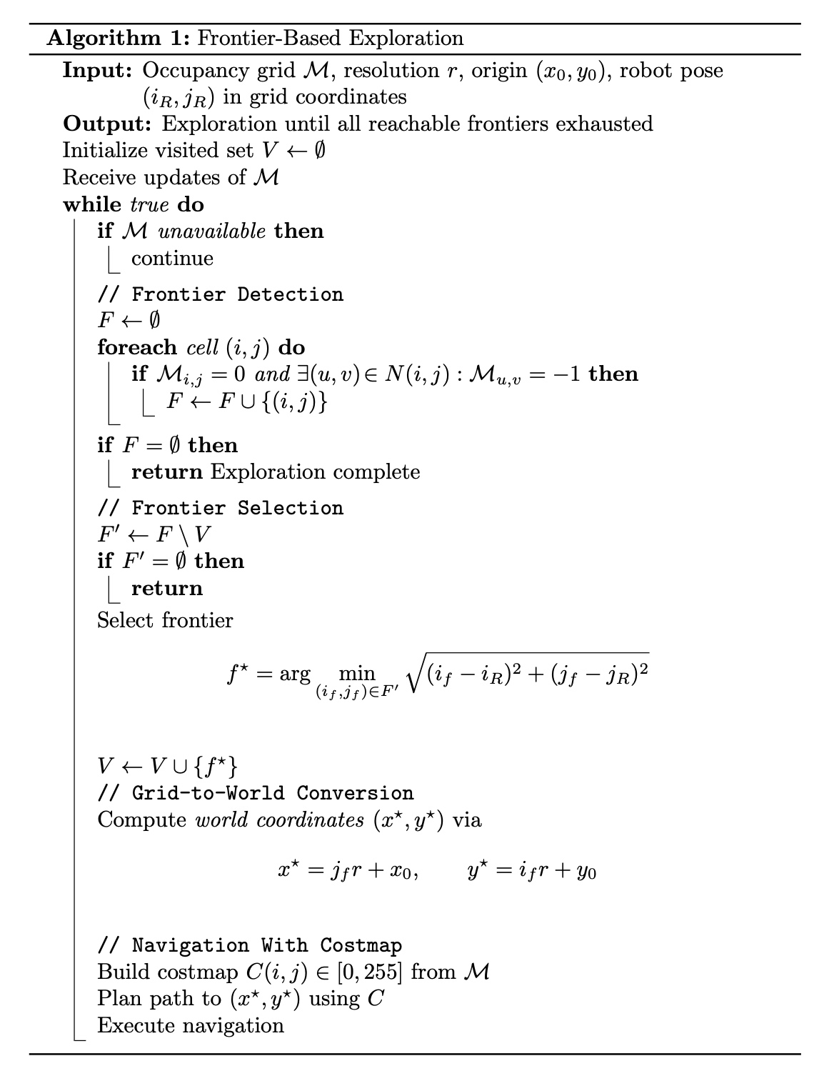
Frontier Explorer
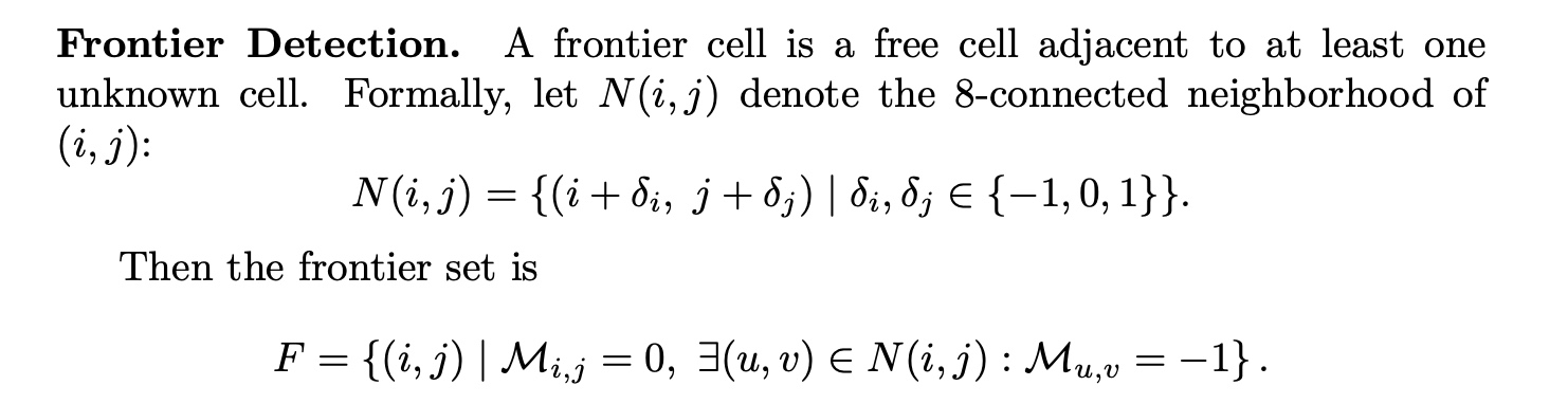
Next, we have the explorer node. The explorer node subscribes to the published occupancy grid and performs frontier-based exploration to autonomously select navigation goals. Frontiers are defined as boundaries between known free space and unknown space in the occupancy grid. The explorer periodically scans the grid to identify these frontiers, clusters nearby frontier cells, and selects a goal based on the shortest euclidean distance to the robot. Once a goal is selected, it is published as a NavigateToPose goal to the Nav2 stack, which handles global path planning, local obstacle avoidance, and trajectory execution.
Going into more details, our explorer node works by first transforming the binary occupancy grid published to /map (which only contains if a cell is free or occupied) into a new model.
Then, it attempts to find frontiers, which are defined as follows:
Finally, we run our frontier-based exploration algorithm, which is defined as follows:
Navigation & Control
When a NavigateToPose goal is sent to Nav2, the navigation stack triggers a coordinated planning and control pipeline. The global planner first computes a collision-free path on the global costmap from the robot’s current pose toward the target goal, producing a sequence of waypoints that avoids known obstacles and respects the environment structure. This planned path is then handed off to the controller server, which operates in the odom frame with the local costmap that incorporates up-to-date sensor information. The local planner’s job is to track this path while reacting to dynamic obstacles and minor changes in the environment, outputting velocity commands at high frequency to smoothly guide the robot along the global plan. These commands are published on the /cmd_vel topic; our cmd_vel_to_go2 node then translates them into the specific control format expected by the Go2 robot, ensuring appropriate scaling and safety limits before sending them to the hardware. This cycle continues until the goal is reached, a timeout or recovery behavior is triggered, or a new goal is received.
For the local control effort, we use Nav2’s Model Predictive Path Integral (MPPI) controller, a modern predictive controller that generalizes traditional Model Predictive Control (MPC) with a sampling-based optimization approach. Instead of following the path point-by-point reactively, the MPPI controller generates many candidate control sequences by sampling perturbations around the robot’s current velocity profile and forward simulating resulting trajectories within its motion model. Each trajectory is evaluated against cost criteria such as path tracking error, obstacle avoidance, and smoothness, and the best sequence guides the robot’s next velocity command. Because MPPI optimizes over a prediction horizon and can incorporate multiple behavioral objectives through plugin-based cost functions, it tends to produce smoother, more adaptive motion in dynamic environments compared to simpler reactive controllers. This controller runs continuously at real-time rates (e.g., dozens of Hz), allowing Nav2 to robustly track the global path while handling unexpected obstacles and kinematic constraints.
Overall, this system cleanly decomposes autonomy into the three required pillars of perception, planning, and actuation, resulting in a clear and extensible architecture. Perception begins with raw LiDAR point clouds published by the Go2 robot, which are transformed and fused into a probabilistic occupancy grid using Bayesian log-odds updates. This map provides a consistent spatial representation of the environment that supports both exploration and navigation. Planning is handled at multiple levels: the frontier-based explorer selects high-level exploration goals that expand known free space, while the Nav2 stack computes global paths on the global costmap and refines them locally using a predictive MPPI controller that accounts for dynamic obstacles and robot kinematics. Finally, actuation is achieved by translating Nav2’s velocity commands into Go2-specific control messages through a dedicated interface node, enabling safe and smooth execution of planned motions on the physical robot. Together, these components form a modular system that satisfies the project requirements while remaining robust to environmental uncertainty and future extensions, such as using some computer vision techniques to identify potential humans or animals and localize them onto the map for search and rescue!